This page is based on the chapter
“Timeseries”
of the Modern Polars book.
Preparing Data
Since the PRQL and SQL results shown on this page are after being
converted to R DataFrame via knitr, they have been converted from DuckDB
types to R types. So NULL in DuckDB is shown as NA.
Download
Download the data from Binance REST
API
and write it to a Parquet file.
This document uses R to download the data from the source here, but we
can also download and use the Parquet file included in the
kevinheavey/modern-polars
GitHub repository.
Code
R
data_path <- "data/ohlcv.parquet"
if (!fs::file_exists(data_path)) {
fs::dir_create(fs::path_dir(data_path))
.epoch_ms <- function(dt) {
dt |>
lubridate::as_datetime() |>
(\(x) (as.integer(x) * 1000))()
}
.start <- lubridate::make_datetime(2021, 1, 1) |> .epoch_ms()
.end <- lubridate::make_datetime(2022, 1, 1) |> .epoch_ms()
.url <- glue::glue(
"https://api.binance.com/api/v3/klines?symbol=BTCUSDT&",
"interval=1d&startTime={.start}&endTime={.end}"
)
.res <- jsonlite::read_json(.url)
time_col <- "time"
ohlcv_cols <- c(
"open",
"high",
"low",
"close",
"volume"
)
cols_to_use <- c(time_col, ohlcv_cols)
cols <- c(cols_to_use, glue::glue("ignore_{i}", i = 1:6))
df <- .res |>
tibble::enframe(name = NULL) |>
tidyr::unnest_wider(value, names_sep = "_") |>
rlang::set_names({{ cols }}) |>
dplyr::mutate(
dplyr::across({{ time_col }}, \(x) lubridate::as_datetime(x / 1000) |> lubridate::as_date()),
dplyr::across({{ ohlcv_cols }}, as.numeric),
.keep = "none"
)
con_tmp <- DBI::dbConnect(duckdb::duckdb(), ":memory:")
duckdb::duckdb_register(con_tmp, "df", df)
duckdb:::sql(glue::glue("COPY df TO '{data_path}' (FORMAT PARQUET)"), con_tmp)
DBI::dbDisconnect(con_tmp)
}
This is a sample command to download the Parquet file from the
kevinheavey/modern-polars GitHub repository.
Terminal
mkdir data
curl -sL https://github.com/kevinheavey/modern-polars/raw/d67d6f95ce0de8aad5492c4497ac4c3e33d696e8/data/ohlcv.pq -o data/ohlcv.parquet
Load the Data
After the Parquet file is ready, load that into DuckDB (in-memory)
database table, R DataFrame, and Python polars.LazyFrame.
- DuckDB
- R DataFrame
- Python polars.LazyFrame
SQL
CREATE TABLE tab AS FROM 'data/ohlcv.parquet'
| 2021-01-01 |
28923.63 |
29600.00 |
28624.57 |
29331.69 |
54182.93 |
| 2021-01-02 |
29331.70 |
33300.00 |
28946.53 |
32178.33 |
129993.87 |
| 2021-01-03 |
32176.45 |
34778.11 |
31962.99 |
33000.05 |
120957.57 |
| 2021-01-04 |
33000.05 |
33600.00 |
28130.00 |
31988.71 |
140899.89 |
| 2021-01-05 |
31989.75 |
34360.00 |
29900.00 |
33949.53 |
116050.00 |
R
library(dplyr, warn.conflicts = FALSE)

df <- duckdb:::sql("FROM 'data/ohlcv.parquet'")
| 2021-01-01 |
28923.63 |
29600.00 |
28624.57 |
29331.69 |
54182.93 |
| 2021-01-02 |
29331.70 |
33300.00 |
28946.53 |
32178.33 |
129993.87 |
| 2021-01-03 |
32176.45 |
34778.11 |
31962.99 |
33000.05 |
120957.57 |
| 2021-01-04 |
33000.05 |
33600.00 |
28130.00 |
31988.71 |
140899.89 |
| 2021-01-05 |
31989.75 |
34360.00 |
29900.00 |
33949.53 |
116050.00 |
Python
import polars as pl

lf = pl.scan_parquet("data/ohlcv.parquet")
shape: (5, 6)
| date |
f64 |
f64 |
f64 |
f64 |
f64 |
| 2021-01-01 |
28923.63 |
29600.0 |
28624.57 |
29331.69 |
54182.925011 |
| 2021-01-02 |
29331.7 |
33300.0 |
28946.53 |
32178.33 |
129993.873362 |
| 2021-01-03 |
32176.45 |
34778.11 |
31962.99 |
33000.05 |
120957.56675 |
| 2021-01-04 |
33000.05 |
33600.0 |
28130.0 |
31988.71 |
140899.88569 |
| 2021-01-05 |
31989.75 |
34360.0 |
29900.0 |
33949.53 |
116049.997038 |
Filtering
- PRQL DuckDB
- SQL DuckDB
- dplyr R
- Python Polars
PRQL
from tab
filter s"date_part(['year', 'month'], time) = {{year: 2021, month: 2}}"
take 5
| 2021-02-01 |
33092.97 |
34717.27 |
32296.16 |
33526.37 |
82718.28 |
| 2021-02-02 |
33517.09 |
35984.33 |
33418.00 |
35466.24 |
78056.66 |
| 2021-02-03 |
35472.71 |
37662.63 |
35362.38 |
37618.87 |
80784.33 |
| 2021-02-04 |
37620.26 |
38708.27 |
36161.95 |
36936.66 |
92080.74 |
| 2021-02-05 |
36936.65 |
38310.12 |
36570.00 |
38290.24 |
66681.33 |
SQL
FROM tab
WHERE date_part(['year', 'month'], time) = {year: 2021, month: 2}
LIMIT 5
| 2021-02-01 |
33092.97 |
34717.27 |
32296.16 |
33526.37 |
82718.28 |
| 2021-02-02 |
33517.09 |
35984.33 |
33418.00 |
35466.24 |
78056.66 |
| 2021-02-03 |
35472.71 |
37662.63 |
35362.38 |
37618.87 |
80784.33 |
| 2021-02-04 |
37620.26 |
38708.27 |
36161.95 |
36936.66 |
92080.74 |
| 2021-02-05 |
36936.65 |
38310.12 |
36570.00 |
38290.24 |
66681.33 |
R
df |>
  filter(
    lubridate::floor_date(time, "month") == lubridate::make_datetime(2021, 2)
  ) |>
  head(5)
| 2021-02-01 |
33092.97 |
34717.27 |
32296.16 |
33526.37 |
82718.28 |
| 2021-02-02 |
33517.09 |
35984.33 |
33418.00 |
35466.24 |
78056.66 |
| 2021-02-03 |
35472.71 |
37662.63 |
35362.38 |
37618.87 |
80784.33 |
| 2021-02-04 |
37620.26 |
38708.27 |
36161.95 |
36936.66 |
92080.74 |
| 2021-02-05 |
36936.65 |
38310.12 |
36570.00 |
38290.24 |
66681.33 |
Python
(
    lf.filter((pl.col("time").dt.year() == 2021) & (pl.col("time").dt.month() == 2))
    .head(5)
    .collect()
)
shape: (5, 6)
| date |
f64 |
f64 |
f64 |
f64 |
f64 |
| 2021-02-01 |
33092.97 |
34717.27 |
32296.16 |
33526.37 |
82718.276882 |
| 2021-02-02 |
33517.09 |
35984.33 |
33418.0 |
35466.24 |
78056.65988 |
| 2021-02-03 |
35472.71 |
37662.63 |
35362.38 |
37618.87 |
80784.333663 |
| 2021-02-04 |
37620.26 |
38708.27 |
36161.95 |
36936.66 |
92080.735898 |
| 2021-02-05 |
36936.65 |
38310.12 |
36570.0 |
38290.24 |
66681.334275 |
Downsampling
It is important to note carefully how units such as 5 days or 1 week
actually work. In other words, where to start counting 5 days or
1 week could be completely different in each system.
Here, we should note that time_bucket in DuckDB,
lubridate::floor_date in R, and group_by_dynamic in Polars have
completely different initial starting points by default.
-
The DuckDB function time_bucket’s origin defaults to
2000-01-03 00:00:00+00 for days or weeks interval.1
-
In the R lubridate::floor_date function, timestamp is floored
using the number of days elapsed since the beginning of every month
when specifying "5 days" to the unit argument.
R
lubridate::as_date(c("2023-01-31", "2023-02-01")) |>
  lubridate::floor_date("5 days")
[1] "2023-01-31" "2023-02-01"
And when "1 week" to the unit argument, it is floored to the
nearest week, Sunday through Saturday.
R
lubridate::as_date(c("2023-01-31", "2023-02-01")) |>
  lubridate::floor_date("1 week")
[1] "2023-01-29" "2023-01-29"
To start from an arbitrary origin, all breaks must be specified as a
vector in the unit argument.2
R
lubridate::as_date(c("2023-01-31", "2023-02-01")) |>
  lubridate::floor_date(lubridate::make_date(2023, 1, 31))
[1] "2023-01-31" "2023-01-31"
-
group_by_dynamic of Polars, the offset parameter to specify the
origin point, is negative every by default.3
- PRQL DuckDB
- SQL DuckDB
- dplyr R
- Python Polars
PRQL
from tab
derive {
  time_new = s"""
    time_bucket(INTERVAL '5 days', time, (FROM tab SELECT min(time)))
  """
}
group {time_new} (
  aggregate {
    open = average open,
    high = average high,
    low = average low,
    close = average close,
    volume = average volume
  }
)
sort time_new
take 5
| 2021-01-01 |
31084.32 |
33127.62 |
29512.82 |
32089.66 |
112416.85 |
| 2021-01-06 |
38165.31 |
40396.84 |
35983.82 |
39004.54 |
118750.08 |
| 2021-01-11 |
36825.23 |
38518.10 |
33288.05 |
36542.76 |
146166.70 |
| 2021-01-16 |
36216.36 |
37307.53 |
34650.37 |
35962.92 |
81236.80 |
| 2021-01-21 |
32721.53 |
34165.71 |
30624.23 |
32077.48 |
97809.66 |
SQL
WITH _tab1 AS (
  FROM tab
  SELECT
    * REPLACE (time_bucket(INTERVAL '5 days', time, (FROM tab SELECT min(time)))) AS time
)

FROM _tab1
SELECT
  time,
  avg(COLUMNS(x -> x NOT IN ('time')))
GROUP BY time
ORDER BY time
LIMIT 5
| 2021-01-01 |
31084.32 |
33127.62 |
29512.82 |
32089.66 |
112416.85 |
| 2021-01-06 |
38165.31 |
40396.84 |
35983.82 |
39004.54 |
118750.08 |
| 2021-01-11 |
36825.23 |
38518.10 |
33288.05 |
36542.76 |
146166.70 |
| 2021-01-16 |
36216.36 |
37307.53 |
34650.37 |
35962.92 |
81236.80 |
| 2021-01-21 |
32721.53 |
34165.71 |
30624.23 |
32077.48 |
97809.66 |
R
df |>
  mutate(
    time = time |>
      (\(x) lubridate::floor_date(x, seq(min(x), max(x), by = 5)))()
  ) |>
  summarise(across(everything(), mean), .by = time) |>
  head(5)
| 2021-01-01 |
31084.32 |
33127.62 |
29512.82 |
32089.66 |
112416.85 |
| 2021-01-06 |
38165.31 |
40396.84 |
35983.82 |
39004.54 |
118750.08 |
| 2021-01-11 |
36825.23 |
38518.10 |
33288.05 |
36542.76 |
146166.70 |
| 2021-01-16 |
36216.36 |
37307.53 |
34650.37 |
35962.92 |
81236.80 |
| 2021-01-21 |
32721.53 |
34165.71 |
30624.23 |
32077.48 |
97809.66 |
Python
(
    lf.sort("time")
    .group_by_dynamic("time", every="5d")
    .agg(pl.col(pl.Float64).mean())
    .head(5)
    .collect()
)
shape: (5, 6)
| date |
f64 |
f64 |
f64 |
f64 |
f64 |
| 2020-12-29 |
29127.665 |
31450.0 |
28785.55 |
30755.01 |
92088.399186 |
| 2021-01-03 |
33577.028 |
36008.464 |
31916.198 |
35027.986 |
127574.470245 |
| 2021-01-08 |
38733.61 |
39914.548 |
34656.422 |
37655.352 |
143777.954392 |
| 2021-01-13 |
36659.63 |
38500.052 |
34539.406 |
37016.338 |
102447.076833 |
| 2021-01-18 |
34933.922 |
36232.334 |
32593.012 |
34357.258 |
103530.722029 |
- PRQL DuckDB
- SQL DukcDB
- dplyr R
- Python Polars
PRQL
from tab
derive {
  time_new = s"""
    time_bucket(INTERVAL '7 days', time, (FROM tab SELECT min(time)))
  """
}
group {time_new} (
  aggregate {
    open_mean = average open,
    high_mean = average high,
    low_mean = average low,
    close_mean = average close,
    volume_mean = average volume,
    open_sum = sum open,
    high_sum = sum high,
    low_sum = sum low,
    close_sum = sum close,
    volume_sum = sum volume
  }
)
sort time_new
take 5
| 2021-01-01 |
32305.78 |
34706.05 |
31021.73 |
33807.14 |
117435.59 |
226140.5 |
242942.3 |
217152.1 |
236650.0 |
822049.1 |
| 2021-01-08 |
37869.80 |
39646.11 |
34623.33 |
37827.52 |
135188.30 |
265088.6 |
277522.7 |
242363.3 |
264792.6 |
946318.1 |
| 2021-01-15 |
36527.89 |
37412.20 |
33961.55 |
35343.85 |
94212.72 |
255695.2 |
261885.4 |
237730.9 |
247406.9 |
659489.0 |
| 2021-01-22 |
31888.55 |
33498.81 |
30424.48 |
32248.01 |
89649.94 |
223219.8 |
234491.7 |
212971.4 |
225736.0 |
627549.6 |
| 2021-01-29 |
34511.48 |
36411.44 |
33450.08 |
35022.31 |
102728.42 |
241580.4 |
254880.1 |
234150.6 |
245156.2 |
719099.0 |
SQL
WITH _tab1 AS (
  FROM tab
  SELECT
    * REPLACE (time_bucket(INTERVAL '7 days', time, (FROM tab SELECT min(time)))) AS time
)

FROM _tab1
SELECT
  time,
  avg(COLUMNS(x -> x NOT IN ('time'))),
  sum(COLUMNS(x -> x NOT IN ('time')))
GROUP BY time
ORDER BY time
LIMIT 5
| 2021-01-01 |
32305.78 |
34706.05 |
31021.73 |
33807.14 |
117435.59 |
226140.5 |
242942.3 |
217152.1 |
236650.0 |
822049.1 |
| 2021-01-08 |
37869.80 |
39646.11 |
34623.33 |
37827.52 |
135188.30 |
265088.6 |
277522.7 |
242363.3 |
264792.6 |
946318.1 |
| 2021-01-15 |
36527.89 |
37412.20 |
33961.55 |
35343.85 |
94212.72 |
255695.2 |
261885.4 |
237730.9 |
247406.9 |
659489.0 |
| 2021-01-22 |
31888.55 |
33498.81 |
30424.48 |
32248.01 |
89649.94 |
223219.8 |
234491.7 |
212971.4 |
225736.0 |
627549.6 |
| 2021-01-29 |
34511.48 |
36411.44 |
33450.08 |
35022.31 |
102728.42 |
241580.4 |
254880.1 |
234150.6 |
245156.2 |
719099.0 |
R
df |>
  mutate(
    time = time |>
      (\(x) lubridate::floor_date(x, seq(min(x), max(x), by = 7)))()
  ) |>
  summarise(
    across(
      everything(),
      list(mean = mean, sum = sum),
      .names = "{.col}_{.fn}"
    ),
    .by = time
  ) |>
  head(5)
| 2021-01-01 |
32305.78 |
226140.5 |
34706.05 |
242942.3 |
31021.73 |
217152.1 |
33807.14 |
236650.0 |
117435.59 |
822049.1 |
| 2021-01-08 |
37869.80 |
265088.6 |
39646.11 |
277522.7 |
34623.33 |
242363.3 |
37827.52 |
264792.6 |
135188.30 |
946318.1 |
| 2021-01-15 |
36527.89 |
255695.2 |
37412.20 |
261885.4 |
33961.55 |
237730.9 |
35343.85 |
247406.9 |
94212.72 |
659489.0 |
| 2021-01-22 |
31888.55 |
223219.8 |
33498.81 |
234491.7 |
30424.48 |
212971.4 |
32248.01 |
225736.0 |
89649.94 |
627549.6 |
| 2021-01-29 |
34511.48 |
241580.4 |
36411.44 |
254880.1 |
33450.08 |
234150.6 |
35022.31 |
245156.2 |
102728.42 |
719099.0 |
Python
(
    lf.sort("time")
    .group_by_dynamic("time", every="1w")
    .agg(
        [
            pl.col(pl.Float64).mean().name.suffix("_mean"),
            pl.col(pl.Float64).sum().name.suffix("_sum"),
        ]
    )
    .head(5)
    .collect()
)
shape: (5, 11)
| date |
f64 |
f64 |
f64 |
f64 |
f64 |
f64 |
f64 |
f64 |
f64 |
f64 |
| 2020-12-28 |
30143.926667 |
32559.37 |
29844.696667 |
31503.356667 |
101711.455041 |
90431.78 |
97678.11 |
89534.09 |
94510.07 |
305134.365123 |
| 2021-01-04 |
36545.192857 |
38563.458571 |
33992.73 |
37280.132857 |
121528.60945 |
255816.35 |
269944.21 |
237949.11 |
260960.93 |
850700.266152 |
| 2021-01-11 |
36694.077143 |
38199.0 |
33664.004286 |
36362.485714 |
128191.382064 |
256858.54 |
267393.0 |
235648.03 |
254537.4 |
897339.67445 |
| 2021-01-18 |
34242.515714 |
35384.095714 |
32179.317143 |
33732.027143 |
91460.990826 |
239697.61 |
247688.67 |
225255.22 |
236124.19 |
640226.935785 |
| 2021-01-25 |
32745.312857 |
34563.677143 |
31249.037143 |
32865.862857 |
106780.501216 |
229217.19 |
241945.74 |
218743.26 |
230061.04 |
747463.508509 |
Upsampling
The way to use a function like generate_series to generate sequential
values and then join them is general-purpose.
In R, we can also use dedicated functions like
timetk::pad_by_time.
- PRQL DuckDB
- SQL DuckDB
- dplyr R
- Python Polars
This example does not work with prql-compiler 0.11.1.
(PRQL/prql#3129)
PRQL
let _tab1 = s"""
  SELECT
    generate_series(
      (SELECT min(time)),
      (SELECT max(time)),
      INTERVAL '6 hours'
    ).unnest() AS time
  FROM tab
"""

from _tab1
join side:left tab (==time)
sort tab.time
select !{tab.time}
take 5
SQL
WITH _tab1 AS (
  SELECT
    generate_series(
      (FROM tab SELECT min(time)),
      (FROM tab SELECT max(time)),
      INTERVAL '6 hours'
    ).unnest() AS time
)

FROM _tab1
LEFT JOIN tab USING (time)
ORDER BY time
LIMIT 5
| 2021-01-01 00:00:00 |
28923.63 |
29600 |
28624.57 |
29331.69 |
54182.93 |
| 2021-01-01 06:00:00 |
NA |
NA |
NA |
NA |
NA |
| 2021-01-01 12:00:00 |
NA |
NA |
NA |
NA |
NA |
| 2021-01-01 18:00:00 |
NA |
NA |
NA |
NA |
NA |
| 2021-01-02 00:00:00 |
29331.70 |
33300 |
28946.53 |
32178.33 |
129993.87 |
R
.grid <- df$time |>
  lubridate::as_datetime() |>
  (\(x) seq(min(x), max(x), by = "6 hours"))() |>
  tibble::tibble(time = _)

.grid |>
  left_join(df, by = "time") |>
  head(5)
| 2021-01-01 00:00:00 |
28923.63 |
29600 |
28624.57 |
29331.69 |
54182.93 |
| 2021-01-01 06:00:00 |
NA |
NA |
NA |
NA |
NA |
| 2021-01-01 12:00:00 |
NA |
NA |
NA |
NA |
NA |
| 2021-01-01 18:00:00 |
NA |
NA |
NA |
NA |
NA |
| 2021-01-02 00:00:00 |
29331.70 |
33300 |
28946.53 |
32178.33 |
129993.87 |
Python
lf.collect().sort("time").upsample("time", every="6h").head(5)
shape: (5, 6)
| date |
f64 |
f64 |
f64 |
f64 |
f64 |
| 2021-01-01 |
28923.63 |
29600.0 |
28624.57 |
29331.69 |
54182.925011 |
| 2021-01-01 |
null |
null |
null |
null |
null |
| 2021-01-01 |
null |
null |
null |
null |
null |
| 2021-01-01 |
null |
null |
null |
null |
null |
| 2021-01-02 |
29331.7 |
33300.0 |
28946.53 |
32178.33 |
129993.873362 |
Window Functions
It is necessary to be careful how the Window function calculates if the
width of the window is less than the specified value.
Moving Average, Cumulative Avarage
PRQL has a dedicated way of applying the window to the entire table. For
the others, use a individual function for each column.
In R, base R have some window functions like cumsum, but none like
cumulative avarage. dplyr complements this with several functions,
including cummean.
Polars does not yet have a dedicated function to compute cumulative
averages, so we must use cumulative sums to compute them.
- PRQL DuckDB
- SQL DuckDB
- dplyr R
- Python Polars
PRQL
from tab
sort this.time
window rolling:28 (
  derive {`28D MA` = average close}
)
window rows:..0 (
  derive {`Expanding Average` = average close}
)
select {
  this.time,
  Raw = close,
  `28D MA`,
  `Expanding Average`
}
take 26..30
| 2021-01-26 |
32467.77 |
35032.87 |
35032.87 |
| 2021-01-27 |
30366.15 |
34860.03 |
34860.03 |
| 2021-01-28 |
33364.86 |
34806.63 |
34806.63 |
| 2021-01-29 |
34252.20 |
34982.36 |
34787.51 |
| 2021-01-30 |
34262.88 |
35056.81 |
34770.02 |
SQL
FROM tab
SELECT
  time,
  close AS "Raw",
  avg(close) OVER (
    ORDER BY time
    ROWS BETWEEN 27 PRECEDING AND CURRENT ROW
  ) AS "28D MA",
  avg(close) OVER (
    ORDER BY time
    ROWS BETWEEN UNBOUNDED PRECEDING AND CURRENT ROW
  ) AS "Expanding Average"
LIMIT 5 OFFSET 25
| 2021-01-26 |
32467.77 |
35032.87 |
35032.87 |
| 2021-01-27 |
30366.15 |
34860.03 |
34860.03 |
| 2021-01-28 |
33364.86 |
34806.63 |
34806.63 |
| 2021-01-29 |
34252.20 |
34982.36 |
34787.51 |
| 2021-01-30 |
34262.88 |
35056.81 |
34770.02 |
R
roll_and_expand <- df |>
  arrange(time) |>
  mutate(
    time,
    Raw = close,
    `28D MA` = close |>
      slider::slide_vec(mean, .before = 27, .complete = TRUE),
    `Expanding Average` = cummean(close),
    .keep = "none"
  )
R
roll_and_expand |>
  slice(26:30)
| 2021-01-26 |
32467.77 |
NA |
35032.87 |
| 2021-01-27 |
30366.15 |
NA |
34860.03 |
| 2021-01-28 |
33364.86 |
34806.63 |
34806.63 |
| 2021-01-29 |
34252.20 |
34982.36 |
34787.51 |
| 2021-01-30 |
34262.88 |
35056.81 |
34770.02 |
Python
close = pl.col("close")

roll_and_expand = lf.sort("time").select(
    [
        pl.col("time"),
        close.alias("Raw"),
        close.rolling_mean(28).alias("28D MA"),
        close.alias("Expanding Average").cum_sum() / (close.cum_count() + 1),
    ]
)
Python
roll_and_expand.head(30).tail(5).collect()
shape: (5, 4)
| date |
f64 |
f64 |
f64 |
| 2021-01-26 |
32467.77 |
null |
33735.354074 |
| 2021-01-27 |
30366.15 |
null |
33615.025357 |
| 2021-01-28 |
33364.86 |
34806.6275 |
33606.398966 |
| 2021-01-29 |
34252.2 |
34982.36 |
33627.925667 |
| 2021-01-30 |
34262.88 |
35056.808214 |
33648.408065 |
Here, DuckDB also calculates avarage for cases where the window width is
less than 28 for the 28D MA column, whereas R
slider::slide_vec(.complete = TRUE) and Polars rolling_mean make
them missing values. If we are using DuckDB and need to make replacement
for NULL, we need to add further processing.
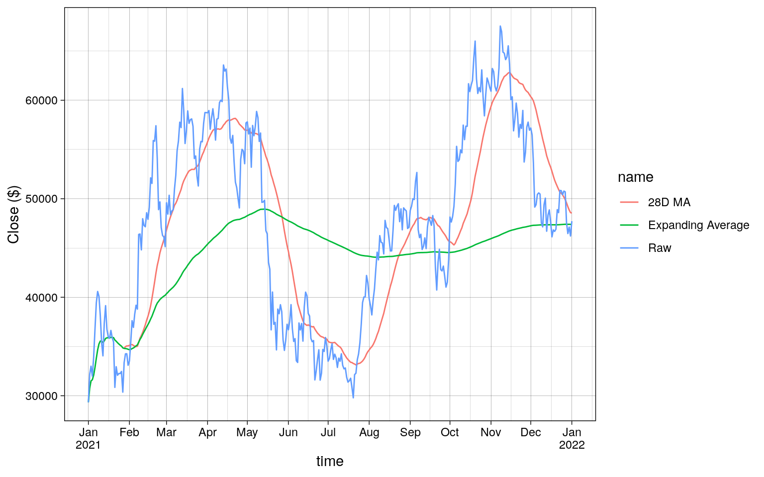
Plotting the results of dplyr shows the following.
Code
R
library(ggplot2)

roll_and_expand |>
  tidyr::pivot_longer(cols = !time) |>
  ggplot(aes(time, value, colour = name)) +
  geom_line() +
  theme_linedraw() +
  labs(y = "Close ($)") +
  scale_x_date(
    date_breaks = "month",
    labels = scales::label_date_short()
  )
Combining Rolling Aggregations
- PRQL DuckDB
- SQL DuckDB
- dplyr R
- Python Polars
PRQL
from tab
sort this.time
window rows:-15..14 (
  select {
    this.time,
    mean = average close,
    std = stddev close
  }
)
take 13..17
| 2021-01-13 |
34860.03 |
3092.516 |
| 2021-01-14 |
34806.63 |
3047.833 |
| 2021-01-15 |
34787.51 |
2994.683 |
| 2021-01-16 |
34770.02 |
2944.156 |
| 2021-01-17 |
34895.40 |
2780.095 |
SQL
FROM tab
SELECT
  time,
  avg(close) OVER (
    ORDER BY time
    ROWS BETWEEN 15 PRECEDING AND 14 FOLLOWING
  ) AS mean,
  stddev(close) OVER (
    ORDER BY time
    ROWS BETWEEN 15 PRECEDING AND 14 FOLLOWING
  ) AS std
ORDER BY time
LIMIT 5 OFFSET 12
| 2021-01-13 |
34860.03 |
3092.516 |
| 2021-01-14 |
34806.63 |
3047.833 |
| 2021-01-15 |
34787.51 |
2994.683 |
| 2021-01-16 |
34770.02 |
2944.156 |
| 2021-01-17 |
34895.40 |
2780.095 |
R
.slide_func <- function(.x, .fn) {
  slider::slide_vec(.x, .fn, .before = 15, .after = 14, .complete = TRUE)
}

mean_std <- df |>
  arrange(time) |>
  mutate(
    time,
    across(
      close,
      .fns = list(mean = \(x) .slide_func(x, mean), std = \(x) .slide_func(x, sd)),
      .names = "{.fn}"
    ),
    .keep = "none"
  )
| 2021-01-13 |
NA |
NA |
| 2021-01-14 |
NA |
NA |
| 2021-01-15 |
NA |
NA |
| 2021-01-16 |
34770.02 |
2944.156 |
| 2021-01-17 |
34895.40 |
2780.095 |
Python
mean_std = lf.sort("time").select(
    time=pl.col("time"),
    mean=pl.col("close").rolling_mean(30, center=True),
    std=pl.col("close").rolling_std(30, center=True),
)
Python
mean_std.head(17).tail(5).collect()
shape: (5, 3)
| date |
f64 |
f64 |
| 2021-01-13 |
null |
null |
| 2021-01-14 |
null |
null |
| 2021-01-15 |
null |
null |
| 2021-01-16 |
34770.021667 |
2944.155675 |
| 2021-01-17 |
34895.398 |
2780.095304 |
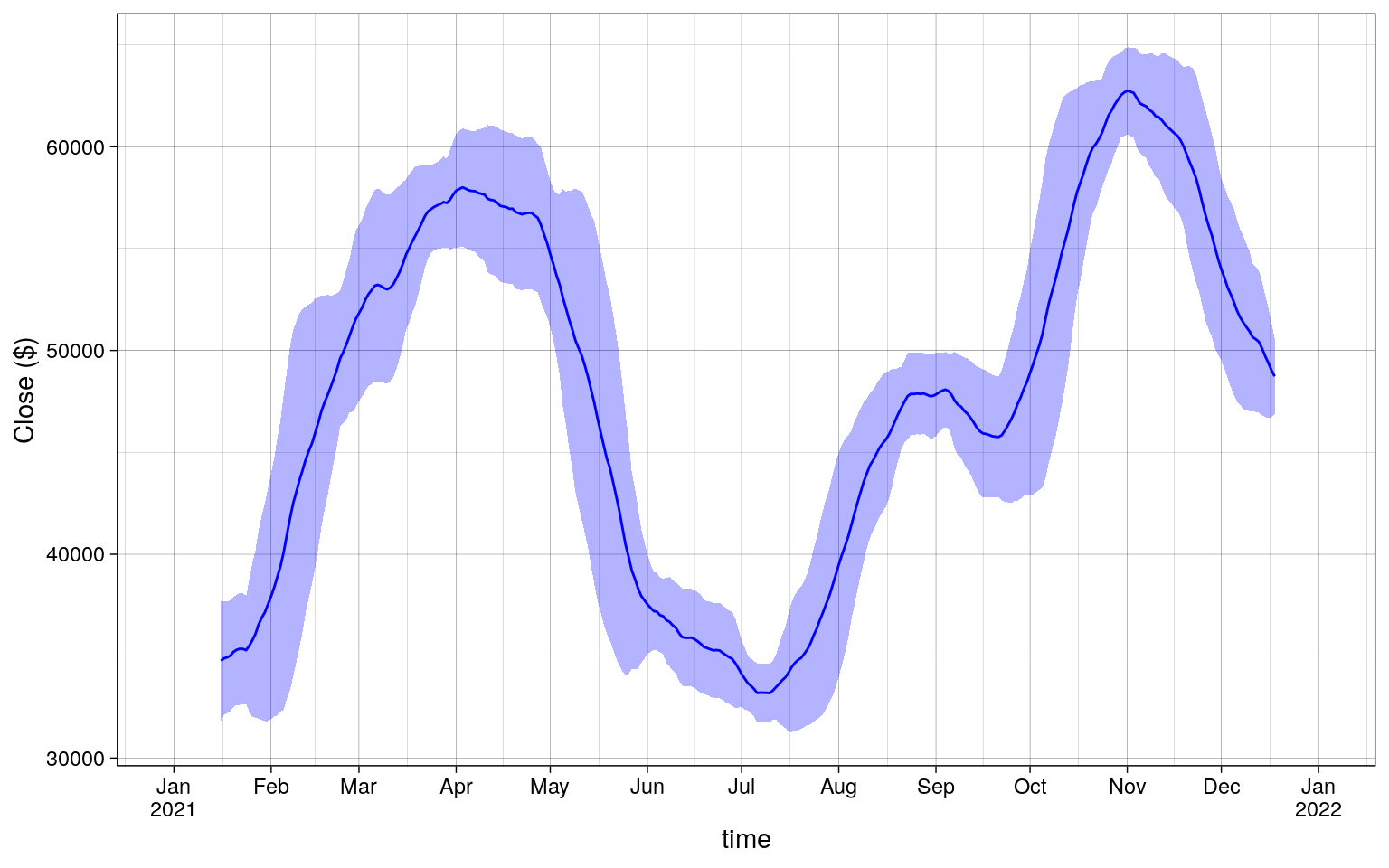
As in Section 5.1,
here too the DuckDB results differ from the others.
Plotting the results of dplyr shows the following.
Code
R
library(ggplot2)

mean_std |>
  ggplot(aes(time)) +
  geom_ribbon(
    aes(ymin = mean - std, ymax = mean + std),
    alpha = 0.3, fill = "blue"
  ) +
  geom_line(aes(y = mean), color = "blue") +
  theme_linedraw() +
  labs(y = "Close ($)") +
  scale_x_date(
    date_breaks = "month",
    labels = scales::label_date_short()
  )
Timezones
In DuckDB, the icu DuckDB extension is needed for time zones support. If
the DuckDB client that we are using does not contain the extension, we
need to install and load it.
- PRQL DuckDB
- SQL DuckDB
- dplyr R
- Python Polars
PRQL
let timezone = tz col -> s"timezone({tz}, {col})"

from tab
derive {
  time_new = (this.time | timezone "UTC" | timezone "US/Eastern")
}
select !{this.time}
take 5
| 28923.63 |
29600.00 |
28624.57 |
29331.69 |
54182.93 |
2020-12-31 19:00:00 |
| 29331.70 |
33300.00 |
28946.53 |
32178.33 |
129993.87 |
2021-01-01 19:00:00 |
| 32176.45 |
34778.11 |
31962.99 |
33000.05 |
120957.57 |
2021-01-02 19:00:00 |
| 33000.05 |
33600.00 |
28130.00 |
31988.71 |
140899.89 |
2021-01-03 19:00:00 |
| 31989.75 |
34360.00 |
29900.00 |
33949.53 |
116050.00 |
2021-01-04 19:00:00 |
SQL
FROM tab
SELECT
  * REPLACE timezone('US/Eastern', timezone('UTC', time)) AS time
LIMIT 5
| 2020-12-31 19:00:00 |
28923.63 |
29600.00 |
28624.57 |
29331.69 |
54182.93 |
| 2021-01-01 19:00:00 |
29331.70 |
33300.00 |
28946.53 |
32178.33 |
129993.87 |
| 2021-01-02 19:00:00 |
32176.45 |
34778.11 |
31962.99 |
33000.05 |
120957.57 |
| 2021-01-03 19:00:00 |
33000.05 |
33600.00 |
28130.00 |
31988.71 |
140899.89 |
| 2021-01-04 19:00:00 |
31989.75 |
34360.00 |
29900.00 |
33949.53 |
116050.00 |
R
df |>
  mutate(
    time = time |>
      lubridate::force_tz("UTC") |>
      lubridate::with_tz("US/Eastern")
  ) |>
  head(5)
| 2020-12-31 19:00:00 |
28923.63 |
29600.00 |
28624.57 |
29331.69 |
54182.93 |
| 2021-01-01 19:00:00 |
29331.70 |
33300.00 |
28946.53 |
32178.33 |
129993.87 |
| 2021-01-02 19:00:00 |
32176.45 |
34778.11 |
31962.99 |
33000.05 |
120957.57 |
| 2021-01-03 19:00:00 |
33000.05 |
33600.00 |
28130.00 |
31988.71 |
140899.89 |
| 2021-01-04 19:00:00 |
31989.75 |
34360.00 |
29900.00 |
33949.53 |
116050.00 |
Python
(
    lf.with_columns(
        pl.col("time")
        .cast(pl.Datetime)
        .dt.replace_time_zone("UTC")
        .dt.convert_time_zone("US/Eastern")
    )
    .head(5)
    .collect()
)
shape: (5, 6)
| datetime[μs, US/Eastern] |
f64 |
f64 |
f64 |
f64 |
f64 |
| 2020-12-31 19:00:00 EST |
28923.63 |
29600.0 |
28624.57 |
29331.69 |
54182.925011 |
| 2021-01-01 19:00:00 EST |
29331.7 |
33300.0 |
28946.53 |
32178.33 |
129993.873362 |
| 2021-01-02 19:00:00 EST |
32176.45 |
34778.11 |
31962.99 |
33000.05 |
120957.56675 |
| 2021-01-03 19:00:00 EST |
33000.05 |
33600.0 |
28130.0 |
31988.71 |
140899.88569 |
| 2021-01-04 19:00:00 EST |
31989.75 |
34360.0 |
29900.0 |
33949.53 |
116049.997038 |
Note that each system may keep time zone information in a different way.
Here, the time column (and the time_new column) in DuckDB results
are the TIMESTAMP type, has no time zone information.